6 Common Hyperparameter Optimization Techniques- NBD Lite #18
Small improvement with big impact to the model...
If you are interested in more audio explanations, you can listen to the article in the AI-Generated Podcast by NotebookLM!👇👇👇
In my opinion, the machine learning model's performance depends mainly on the excellent quality of the data.
That’s why we should always have the best data before anything else.
However, we can still improve the model performance via hyperparameter optimization.
Hyperparameter Optimization is a step to enhance model performance by fine-tuning the settings that govern the learning process.
Unlike model parameters, which are learned directly from the training data, hyperparameters are external settings that must be set before the training begins.
We can have the best model by selecting the most optimum set of hyperparameters and the quality data.
In this post, we will discuss common hyperparameter optimization techniques further.
Below is the visualization to help you understand the hyperparameter optimization 👇👇👇
1. Grid Search
Grid search is a hyperparameter optimization technique with a systematic approach.
The grid in the name refers to the combination of every hyperparameter value we want to try exhaustively.
For example, here is the hyperparameter grid.
param_grid = {
    'n_estimators': [50, 100, 200],
    'max_depth': [None, 10, 20, 30],
    'min_samples_split': [2, 5, 10],
    'min_samples_leaf': [1, 2, 4]
}
From the grid above, we would try every combination available and evaluate the model to find the optimum hyperparameters set.
If we implement it in Python, we could use the following code.
from sklearn.model_selection import GridSearchCV

# Initialize GridSearchCV
grid_search = GridSearchCV(estimator=model,
                           param_grid=param_grid,
                           cv=5,
                           n_jobs=-1,
                           verbose=2,
                           scoring='accuracy')

# Perform Grid Search
grid_search.fit(X_train, y_train)
There are some pros to use Grid Search, including:
Easy to implement and understand.
All specified combinations are considered.
Evaluations can be performed in parallel to speed up the process.
However, there are several cons for using grid search:
It is computationally expensive as the number of combinations grows exponentially with the number of hyperparameters.
It is inefficient as it may spend resources evaluating less promising regions of the hyperparameter space.
Overall, Grid Search is suitable when the number of hyperparameter spaces is small and used as a baseline comparison before we move to a more advanced technique.
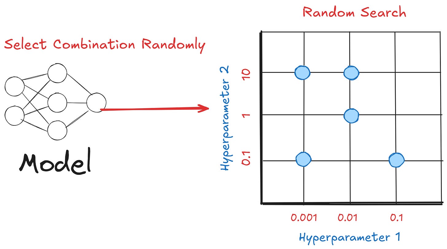
2. Random Search
Random Search is a hyperparameter optimization technique that selects hyperparameter combinations randomly from the grid space.
Unlike Grid Search, it only samples a specified number of configurations for the model evaluation.
Like the Grid Search, we can implement the Random Search with Python.
from sklearn.model_selection import RandomizedSearchCV

random_search = RandomizedSearchCV(estimator=rf,
                                   param_distributions=param_grid,
                                   n_iter=50,
                                   cv=5,
                                   random_state=42,
                                   n_jobs=-1,
                                   verbose=2,
                                   scoring='accuracy')
What is important in the Random Search is the n_iter to control the number of random samples.
There are some pros to use random search, including:
It is efficient as it might be able to find good hyperparameters with fewer iterations.
It can act as the baseline hyperparameter before moving on to the other techniques.
Handles high-dimensional hyperparameter spaces better
However, there are several cons for using random search:
The result can vary due to randomness.
Not cover the entire hyperparameter space.
Random search is best when we are dealing with many hyperparameter combinations and want to limit our computational resources. It’s also good for identifying promising hyperparameter regions.
3. Bayesian Optimization
Bayesian optimization is a hyperparameter optimization technique that uses a probabilistic model approach from Bayesian statistics.
It works by building a probabilistic model of the objective function and iteratively improves this model based on past evaluations.
The key components of Bayesian Optimization are:
Objective Function that represents the error or loss which the technique tries to minimize. (or optimize)
The Surrogate Model, or probabilistic model, approximates the objective function. You can select any model, but often it is the Gaussian Process (GP).
Acquisition Function, which is the function of determining the next set of hyperparameters to evaluate.
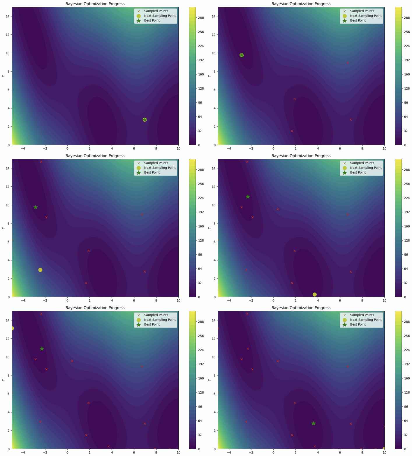
Bayesian optimization method can be summarized in the visualization below.
In a simplified explanation, Bayesian Optimization uses the surrogate model to map the objective function in the hyperparameter space. Rather than using every hyperparameter combination, only a few samples are used to approximate the true objective function.
Then, the process is repeated using the acquisition function to find the next set of hyperparameters until the approximation is optimal. Ultimately, we get the hyperparameters representing the best objective function.
It sounds wordy—basically, bayesian optimization searches for the best hyperparameters using a probabilistic model to guide exploration based on past evaluations of an objective function and acquisition function.
As for the Python implementation, we can use the bayesian-optimization package.
!pip install bayesian-optimizationThen, use the following code for the Bayesian optimization implementation.
from bayes_opt import BayesianOptimization

# Define the objective function
def objective_function(x, y):
    return -((4 - 2.1 * x**2 + (x**4) / 3) * x**2 + x * y + (-4 + 4 * y**2) * y**2)

# Set the hyperparameter space
pbounds = {'x': (-3, 3), 'y': (-2, 2)}

optimizer = BayesianOptimization(
    f=objective_function,
    pbounds=pbounds,
    random_state=42,
)

optimizer.maximize(
    init_points=5,  # Number of initial random evaluations
    n_iter=15       # Number of iterations for optimization
   acq='ei'         # Acquisition Function
)
Change your objective function and acquisition function to experiment with the process.
There are some pros to using Bayesian optimization, including:
It’s able to find near-optimal hyperparameters with fewer iterations.
Able to incorporate uncertainty from the surrogate model.
Adapt based on the new data.
However, there are several cons for using Bayesian optimization:
Much more complex to understand.
It can be computationally expensive.
Would struggle in high-dimensional hyperparameter space.
Bayesian optimzation is good to use when each model evaluation for hyperparameter optimization cost is high, and we want to minimize the number of iterations.
4. Hyperband
Hyperband is a hyperparameter optimization that aims to allocate computational resources efficiently.
It combines the principles of random search, bandit-based, and successive halving.
Mainly there are 4 steps for Hyperbands:
Define Maximum Resources and Minimum Resource
Set the highest and lowest amounts of computational budget (e.g., epochs) to allocate per hyperparameter configuration.
Determine the Number of Brackets
Calculate the different allocation strategies by determining how many brackets (iterations) are needed based on the resource limits.
Perform Successive Halving
Iteratively evaluate and progressively retain only the top-performing configurations within each bracket by allocating increasing resources.
Aggregate Results Across Brackets
Combine the best configurations from all brackets to identify and select the optimal hyperparameter set.
For a simple illustration, imagine we have a deep learning model where we train them for 10 epochs. Hyperband might done the following:
Start by training 81 different hyperparameter configurations for 1 epoch each.
Select the top 27 configurations and train them for 3 epochs each.
Select the top 9 configurations and train them for 9 epochs each.
Finally, select the top 3 configurations and train them for the full 27 epochs.
With Python, we can use the following code to perform Hyperband
from sklearn.experimental import enable_halving_search_cv
from sklearn.model_selection import HalvingRandomSearchCV, StratifiedKFold

# Define the cross-validation strategy
cv = StratifiedKFold(n_splits=3, shuffle=True, random_state=42)

halving_search = HalvingRandomSearchCV(
    estimator=model,
    param_distributions=param_grid,
    factor=3,                   # Reduction factor
    resource='n_estimators',    # Resource to increment
    max_resources=500,          # Maximum resource
    cv=cv,
    scoring='accuracy',
    verbose=1,
    n_jobs=-1,
    random_state=42
)

halving_search.fit(X, y)
There are some pros to using Hyperbands, including:
Efficiently balances exploration and exploitation.
Scales well with large hyperparameter spaces.
However, there are several cons for using Hyperbands:
Requires careful setting of resource allocation parameters
It may not capture dependencies between hyperparameters effectively.
Hyperband is useful when dealing with many hyperparameter configurations and limited computational resources, and we want to efficiently allocate more resources to the most promising settings.
5. Genetic Algorithm
Genetic Algorithm or Evolutionary algorithm is a hyperparameter optimization technique based on evolution.
It would try to mimic the process by representing a set of hyperparameters as an individual within the population.
In general, the steps for the Genetic Algorithm are:
Generate a randomly sampled population (hyperparameters) where this is generation 0.
Evaluate the fitness value (metrics) of each individual in the population in terms of machine learning and get the cross-validation scores.
Generate a new generation using genetic operators (Crossover, Elitism, Mutation).
Repeat until meeting the stopping criterion.
For Python implementation, we can use the deep package.
pip install deapThere are some pros to using Genetic Algorithms, including:
Capable of navigating complex, high-dimensional search spaces.
Good at escaping local optima.
However, there are several cons for using Genetic Algorithms:
It is computationally intensive as it requires many evaluations over generations.
Parameter settings for the algorithm itself (e.g., mutation rate) can be tricky to choose.
Genetic Algorithms are useful when the hyperparameter landscape is highly non-convex or has many local optima, basically if we know that our model is stuck in the same place without increasing their performance.
6. AutoML Frameworks
AutoML is a framework that automates the process of machine learning pipeline development, including hyperparameter optimization.
AutoML is not necessarily the singular technique for hyperparameter optimization.
Instead, it would help us automatically integrate all the techniques we have learned above within the automated workflow.
There are many AutoML frameworks to try, such as TPOT.
pip install tpotThere are some pros to using AutoML frameworks, including:
Easy to use.
Comprehensive as it’s a whole machine learning pipeline automation.
However, there are several cons for using AutoML frameworks:
It can be computationally expensive.
Less control and might not understand the hyperparameter optimization technique were used.
Ultimately, the AutoML framework for hyperparameter optimization is better if we need a quick model building without depth tuning.
That’s all for today! I hope this helps you understand some of the common hyperparameter optimizations.
Are there any more things you would love to discuss? Let’s talk about it together!
👇👇👇
Previous NBD Lite Series
Don’t forget to share Non-Brand Data with your colleagues and friends if you find it useful!


