


Analyzing Time Series Data with Python and Spark
Small Data to Big Data: Scaling Time Series Analysis Seamlessly


Time-series data—records indexed by timestamps—is the foundation of many fields, including finance, tech, and science. Data such as stock prices, IoT sensor streams, or weather forecasts are recorded in a time series manner and reveal how metrics evolve.
Raw time-series data is rarely straightforward. Hidden within the data are patterns such as seasonal rhythms, long-term trends, and noise that muddies the signal.
Moreover, scaling analysis to massive datasets—like billions of sensor readings—adds another layer of complexity.
This is where Python and Apache Spark, a distributed engine for crunching petabytes of data across clusters, can help solve the problem. Together, they transform the data into insight.
This article will teach us more about implementing time-series analysis with Python and Spark. Are you curious about it? Let’s explore it further.
Basics of Time-Series Analysis⏳
We understand that timestamps index the time-series data, but it was much more. In general, four core components govern time series data:
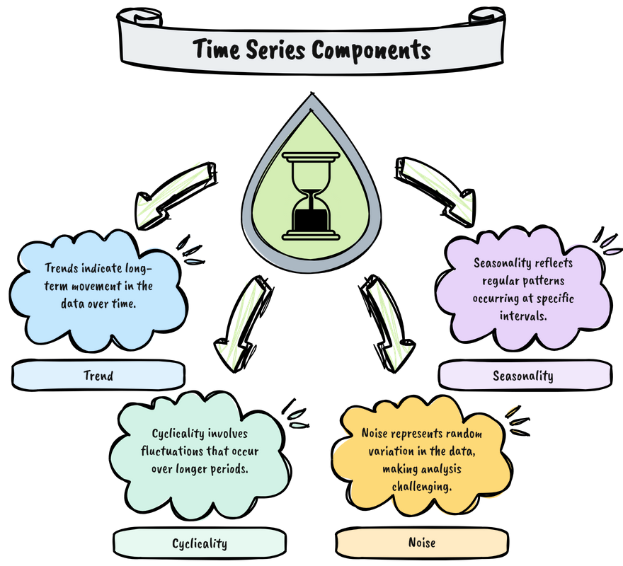
#1. Trend
The trend is the persistent, long-term movement in time-series data, revealing whether values rise, fall, or stabilize over time. For example, the gradual increase in global average temperatures reflects climate change trends, despite short-term fluctuations like seasonal cooling.
#2. Seasonality
Seasonality refers to predictable, repeating patterns tied to fixed intervals, such as daily, weekly, or yearly cycles. For example, holiday sales surge every December, or energy consumption peaks on weekday mornings as people start their days.
#3. Cyclicality
Cyclicality is an irregular, long-term fluctuation often influenced by external forces like economic policies or market sentiment. Unlike seasonality, cycles, such as real estate markets driven by interest rates and consumer confidence, lack fixed timing.
#4. Noise
Noise is the random or unexplainable variation in data, usually caused by measurement errors, outliers, or one-off events. For example, a sudden sensor malfunction might record a false temperature spike, or a viral post might briefly spike app downloads.
These four components are important parts of time-series analysis as they provide insight into the dataset. But how can we analyze them?
We use Python to analyze the time-series data and break down the necessary components to acquire information.
Python Implementation: Step-by-Step Example👨💻
Let’s see how to analyze the time-series data and break down the time-series component with Python code.
For example, we generated a synthetic daily time-series data about temperature fluctuation.
import pandas as pd
import numpy as np

dates = pd.date_range(start="2023-01-01", periods=365, freq="D")

trend = 0.05 * np.arange(365)
seasonality = 10 * np.sin(2 * np.pi * np.arange(365)/365 * 30)
noise = np.random.normal(0, 2, 365)

temperature = 20 + trend + seasonality + noise

df = pd.DataFrame({
    'date': dates,
    'temperature': temperature
}).set_index('date')
It will look like this if we visualize the temperature data.
import matplotlib.pyplot as plt

plt.figure(figsize=(12, 6))
plt.plot(df.index, df['temperature'], label='Daily Temperature')
plt.title("Synthetic Temperature Data")
plt.xlabel("Date")
plt.ylabel("°C")
plt.grid(True)
plt.legend()
plt.show()
Then, if we decomposed the time series data, it will

If we decompose the data above into various components, we can use the statsmodels.
from statsmodels.tsa.seasonal import seasonal_decompose

result = seasonal_decompose(df['temperature'], model='additive', period=30)

plt.figure(figsize=(12, 8))
result.plot()
plt.tight_layout()
plt.xticks(rotation = 90)
plt.show()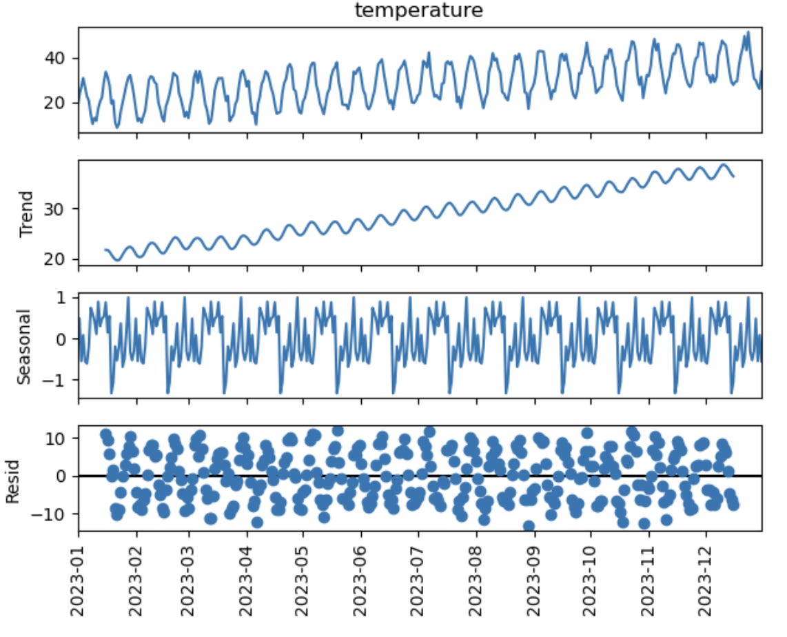
The decomposition above confirms that:
There has been a steady increase throughout the year.
The temperature also exhibits a consistent periodic cycle around that rising baseline.
After removing trend and seasonality, the leftover noise looks fairly random, which is typically what you want to see in a well-decomposed time series.
You can decide which action to take based on the insight above. That's the beauty of time-series analysis, as the insight is often explainable enough to the user.
Scaling with Apache Spark📈
Apache Spark is an open-source, distributed computing framework designed to process massive datasets quickly and efficiently.
Unlike traditional single-node tools (e.g., Pandas), Spark splits data and computations across clusters of machines. This mechanism allows Apache Spark to handle petabyte-scale workloads—from IoT sensor networks to financial market data—often resembling time series data.
Let’s try it out with the Python code for using Apache Spark.
First, we will simulate the temperature data similarly to before. However, we will add a simulated condition where 10,000 devices take the temperature.
import pandas as pd
import numpy as np

dates = pd.date_range(start="2023-01-01", periods=365, freq="D")
base_trend = 0.05 * np.arange(365)
base_seasonality = 10 * np.sin(2 * np.pi * np.arange(365)/365 * 30)
noise = np.random.normal(0, 2, 365)
base_temp = 20 + base_trend + base_seasonality + noise

devices = [f"device_{i}" for i in range(10000)]
data = []

for device in devices:
    # Add device-specific noise (±1°C)
    device_noise = np.random.normal(0, 1, 365)
    device_temp = base_temp + device_noise

    for day, temp in zip(dates, device_temp):
        data.append({
            "device_id": device,
            "timestamp": day,
            "temperature": round(temp, 2)
        })

pdf = pd.DataFrame(data)
The dataset is then converted into a Spark DataFrame.
from pyspark.sql import SparkSession

spark = SparkSession.builder \
    .appName("SyntheticTimeSeries") \
    .getOrCreate()

sdf = spark.createDataFrame(pdf)
Once the dataset is ready, we can perform time-series analysis with Spark. For example, we can perform rolling windows analysis to smooth data.
from pyspark.sql.window import Window
from pyspark.sql.functions import avg, col

window_spec = Window \
    .partitionBy("device_id") \
    .orderBy("timestamp") \
    .rowsBetween(-6, 0)  # 7-day window

sdf_rolling = sdf.withColumn("7_day_avg", avg(col("temperature")).over(window_spec))

sdf_rolling.filter(col("device_id").isin(["device_1", "device_2", "device_3"])) \
    .orderBy("device_id", "timestamp") \
    .show(10)
The smoothing data is swiftly performed on 10,000 different devices, resulting in a table similar to the one above. That’s how powerful Spark is in processing big data.
🔥If you are serious about implementing Spark in your Pipeline or want to enhance that portfolio, I recommend you…
𝐓𝐢𝐦𝐞 𝐒𝐞𝐫𝐢𝐞𝐬 𝐀𝐧𝐚𝐥𝐲𝐬𝐢𝐬 𝐰𝐢𝐭𝐡 𝐒𝐩𝐚𝐫𝐤 by Yoni Ramaswami👋
𝐋𝐞𝐭 𝐦𝐞 𝐭𝐞𝐥𝐥 𝐲𝐨𝐮 𝐰𝐡𝐲 𝐈 𝐫𝐞𝐜𝐨𝐦𝐦𝐞𝐧𝐝 𝐭𝐡𝐢𝐬 𝐛𝐨𝐨𝐤!
🔍 𝐖𝐡𝐚𝐭’𝐬 𝐈𝐧𝐬𝐢𝐝𝐞?
This book is essential if you want to improve your time series skills. It guides building, scaling, and deploying time series pipelines using Spark.
𝐅𝐫𝐨𝐦 𝐙𝐞𝐫𝐨 𝐭𝐨 𝐏𝐫𝐨𝐝𝐮𝐜𝐭𝐢𝐨𝐧: Starts with the basics but quickly explores real-world workflows. I loved the chapters on the End-to-End View of a Time Series Analysis Project.
𝐔𝐬𝐞𝐟𝐮𝐥 𝐒𝐩𝐚𝐫𝐤 𝐈𝐦𝐩𝐥𝐞𝐦𝐞𝐧𝐭𝐚𝐭𝐢𝐨𝐧: This guide doesn’t just explain Spark’s APIs and how to use Delta Lake for data versioning, MLflow for tracking models, and even generative AI.
𝐏𝐫𝐚𝐜𝐭𝐢𝐜𝐚𝐥 𝐂𝐨𝐝𝐞: The examples aren’t theoretical. You’ll find full workflows for retail inventory forecasting, financial fraud detection, and more.
📌 𝐌𝐲 𝐅𝐚𝐯𝐨𝐫𝐢𝐭𝐞 𝐏𝐚𝐫𝐭: The chapter on "Going to Production" (Chapter 9). It’s rare to find a book that doesn’t gloss over the hard parts—like monitoring drift, retraining models, and securing pipelines.
If you are interested, grab the book here!
Don’t miss the chance to learn one of the most useful tools in the industry!
Special thanks to the Author Yoni Ranaswami, Ankur Mulasi, and Packt to allow this book to exist.