Categorical Feature Selection via Chi-Square

Analyze and selecting your categorical features for creating a prediction model

Mar 16, 2020

In our everyday data science work, we often encounter categorical features. Some people would be confused about how to handle these features, especially when we want to create a prediction model where those models basically an equation that accepting number; not a category.

One way is to encode all the category variable using the OneHotEncoding method (encode all the categorical class into numerical values 0 and 1, where 0 mean absent and 1 is present).

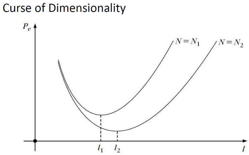
This method is preferable by many as the information is still present and it is easy to understand the concept. The downfall is when we possess many categorical features with high cardinality, the number of the features after OneHotEncoding process would be massive. Why we do not want a lot of features in our training dataset? it is because of the curse of dimensionality.

While adding features could decrease the error in our prediction model, it would only decrease until a certain number of features; after that, the error will increase again. This is the concept of the curse of dimensionality.

Many ways to alleviate this problem, but one of my to-go techniques is by doing feature selection via the Chi-Square test of independence.

Chi-Square Test of Independence

The Chi-Square test of independence is used to determine if there is a significant relationship between two categorical (nominal) variables. It means the Chi-Square Test of Independence is a hypothesis testing test with 2 hypotheses present; the Null Hypothesis and the Alternative Hypothesis. The hypothesis is written below.

Null Hypothesis (H0): There is no relationship between the variables

Alternative Hypothesis (H1): There is a relationship between variables

Just like any statistical testing, we test it against our chosen p-value (often it is 0.05). If the p-value is significant, we can reject the null hypothesis and claim that the findings support the alternative hypothesis. I would not dwell much into the statistic theory, as the purpose of this article is to show how the feature selection using the Chi-Square test is works for practical use.

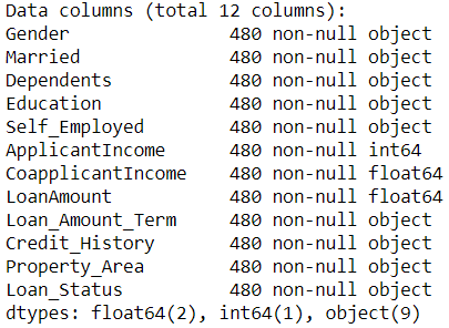
As an example, I would work with a loan dataset from Kaggle for classification problems. Here, the dataset including various numerical, ordinal and nominal variables as stated below (for article purposes, I would drop all the Null values which actually need another analysis).

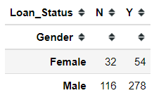
import pandas as pdloan = pd.read_csv('loan_data_set.csv')

#Dropping the uninformative featureloan.drop('Loan_ID')

#Transform the numerical feature into categorical featureloan['Loan_Amount_Term'] = loan['Loan_Amount_Term'].astype('object')loan['Credit_History'] = loan['Credit_History'].astype('object')

#Dropping all the null valueloan.dropna(inplace = True)

#Getting all the categorical columns except the targetcategorical_columns = loan.select_dtypes(exclude = 'number').drop('Loan_Status', axis = 1).columns

loan.info()

In the Chi-Square test, we display the data in a cross-tabulation (contingency) format with each row representing a level (group) for one variable and each column representing a level (group) for another variable. Let’s try to create a cross-tabulation table between Gender and Loan_Status columns.

pd.crosstab(loan['Gender'], loan['Loan_Status'])

Now, let’s try to use the Chi-Square test of independence to test the relationship between these 2 features. Luckily python library scipy already contains the test function for us to use.

# Import the functionfrom scipy.stats import chi2_contingency

#Testing the relationshipchi_res = chi2_contingency(pd.crosstab(loan['Loan_Status'], loan['Gender']))

print('Chi2 Statistic: {}, p-value: {}'.format(chi_res[0], chi_res[1]))

If we choose our p-value level to 0.05, as the p-value test result is more than 0.05 we fail to reject the Null Hypothesis. This means, there is no relationship between the Gender and Loan_Status feature based on the Chi-Square test of independence.

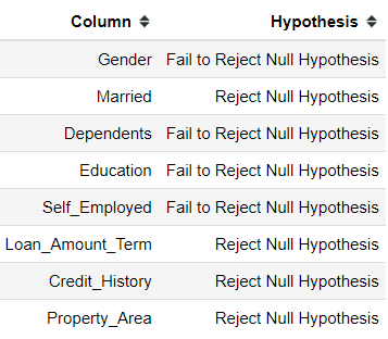
We could try to use this test with all the categorical features present.

chi2_check = []for i in categorical_columns:    if chi2_contingency(pd.crosstab(loan['Loan_Status'], loan[i]))[1] < 0.05:        chi2_check.append('Reject Null Hypothesis')    else:        chi2_check.append('Fail to Reject Null Hypothesis')

res = pd.DataFrame(data = [categorical_columns, chi2_check]              ).T res.columns = ['Column', 'Hypothesis']print(res)

Result of all the Chi-Square test of Independence to all the categorical features

Post Hoc Testing

The Chi-square test of independence is an omnibus test which means it tests the data as a whole. If we have multiple classes within a category, we would not be able to easily tell which class of the features are responsible for the relationship if the Chi-square table is larger than 2×2. To pinpoint which class is responsible, we need a post hoc test.

To conduct multiple 2×2 Chi-square test of independence, we need to regroup the features for each test to where it is one category class against the rest. To do this, we could apply OneHotEncoding to each class and create a new cross-tab table against the other feature.

For example, let’s try to do a post hoc test to the Property_Area feature. First, we need to done OneHotEncoding to the Property_Area feature.

property_dummies = pd.get_dummies(data = loan[['Property_Area', 'Loan_Status']], columns = ['Property_Area'])

Next, we create the cross-tab table for each of the Property_Area class against the target Loan_Status.

#Examplepd.crosstab(property_dummies['Loan_Status'], property_dummies['Property_Area_Rural'])

We then could do a Chi-Square test of independence to this pair.

However, there is something to remember. Comparing multiple classes against each other would means that the error rate of a false positive compound with each test. For example, if we choose our first test at p-value level 0.05 means there is a 5% chance of a false positive; if we have multiple classes, the test after that would compounding the error with the chance become 10% of a false positive, and so forth. With each subsequent test, the error rate would increase by 5%. In our case above, we had 3 pairwise comparisons. This means that our Chi-square test would have an error rate of 15%. Meaning our p-value being tested at would equal 0.15, which is quite high.

In this case, we could use the Bonferroni-adjusted method for correcting the p-value we use. We adjust our P-value by the number of pairwise comparisons we want to do. The formula is p/N, where p= the p-value of the original test and N= the number of planned pairwise comparisons. For example, in our case, above we have 3 class within the Property_Area feature; which means we would have 3 pairwise comparisons if we test all the class against the Loan_Status feature. Our P-value would be 0.05/3 = 0.0167

Using the adjusted P-value, we could test all the previously significant result to see which class are responsible for creating a significant relationship.

check = {}for i in res[res['Hypothesis'] == 'Reject Null Hypothesis']['Column']:    dummies = pd.get_dummies(loan[i])    bon_p_value = 0.05/loan[i].nunique()    for series in dummies:        if chi2_contingency(pd.crosstab(loan['Loan_Status'], dummies[series]))[1] < bon_p_value:            check['{}-{}'.format(i, series)] = 'Reject Null Hypothesis'        else:            check['{}-{}'.format(i, series)] = 'Fail to Reject Null Hypothesis'

res_chi_ph = pd.DataFrame(data = [check.keys(), check.values()]).Tres_chi_ph.columns = ['Pair', 'Hypothesis']res_chi_ph

Here I also include the binary feature for pairwise comparison. As we can see, many of the classes are not actually significant. Even the Loan_Amount_Term that previously significant before the post hoc test resulted in all the classes are not significant.

Prediction Model

The aim of this feature selection technique is to see how it impact our prediction model. Let’s use the simplest model; Logistic Regression as a benchmark. First, I would use all the data and see the model performance in the initial phase. Here, I treat all the categorical data as nominal (even the ordinal data).

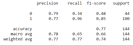
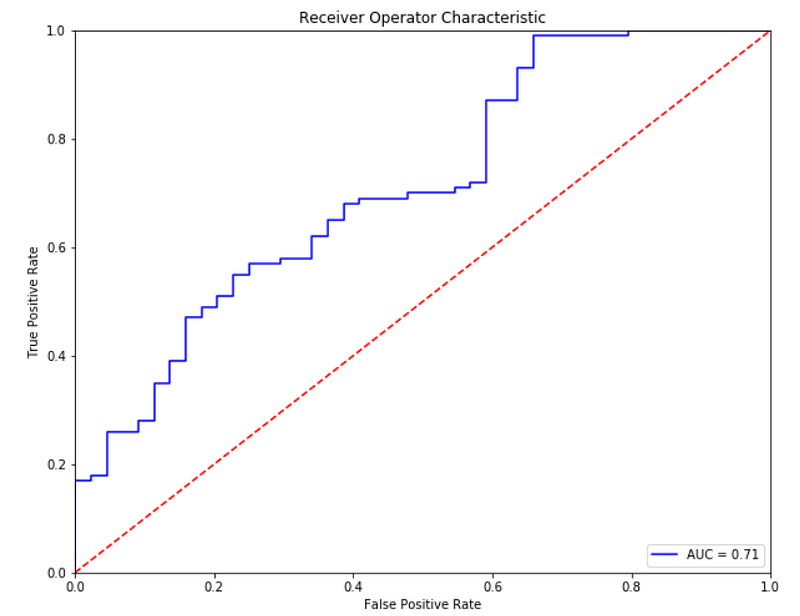
#OneHotEncoding all the categorical variable except the target; Also drop_first = True to avoid multicollinearity for Logistic Regression

data_log = pd.get_dummies(data = loan, columns = loan.select_dtypes(exclude = 'number').drop('Loan_Status', axis =1).columns, drop_first =True)

#Change the class into numerical value

data_log['Loan_Status'] = data_log['Loan_Status'].apply(lambda x: 0 if x == 'N' else 1)

#Splitting the data into Training and Test data

from sklearn.model_selection import train_test_splitX_train, X_test, y_train, y_test = train_test_split(data_log.drop('Loan_Status', axis =1), data_log['Loan_Status'], test_size = 0.30, random_state = 101)

#Creating the prediction modelfrom sklearn.linear_model import LogisticRegressionlog_model = LogisticRegression(max_iter = 1000)log_model.fit(X_train, y_train)

#Performance Checkfrom sklearn.metrics import classification_report, confusion_matrix, roc_curve,auc, accuracy_score

predictions = log_model.predict(X_test)print(accuracy_score(y_test, predictions))Out: 0.7708333333333334

print(classification_report(y_test,predictions))

#Creating the ROC-AUC plot

preds = log_model.predict_proba(X_test)[:,1]fpr, tpr, threshold = roc_curve(y_test, preds)roc_auc = auc(fpr, tpr)plt.figure(figsize=(10,8))plt.title('Receiver Operator Characteristic')plt.plot(fpr, tpr, 'b', label = 'AUC = {}'.format(round(roc_auc, 2)))plt.legend(loc = 'lower right')plt.plot([0,1], [0,1], 'r--')plt.xlim([0,1])plt.ylim([0,1])plt.ylabel('True Positive Rate')plt.xlabel('False Positive Rate')plt.show()

ROC-AUC for the model with all the data as training data

Above is the model performance if we use all the data, let’s compare it with the data we selecting via the Chi-Square Test of Independence.

#Get the list of all the significant pairwise

significant_chi = []for i in res_chi[res_chi['Hypothesis'] == 'Reject Null Hypothesis']['Pair']:    significant_chi.append('{}_{}'.format(i.split('-')[0],i.split('-')[1]))

#Drop the data with duplicate information

for i in ['Married_No', 'Credit_History_0.0']:    significant_chi.remove(i)

#Including the numerical data, as I have not analyze any of this feature

for i in loan.select_dtypes('number').columns:    significant_chi.append(i)

print(significant_chi)

Out: ['Married_Yes', 'Credit_History_1.0','Property_Area_Semiurban', 'ApplicantIncome','CoapplicantIncome', 'LoanAmount']

Previously, if we use all the data as it is we would end up with 21 independent variables. With feature selection, we only have 6 features to work with. I would not do the train test splitting once more because I want to test the data with the same training data and test data. Let’s see how our model performance is with these selected features.

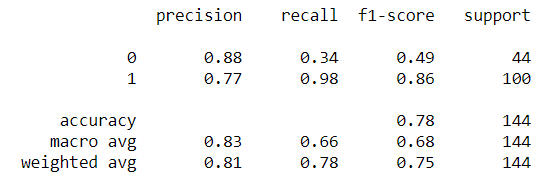
#Training the model only with the significant features and the numerical features

log_model = LogisticRegression(max_iter = 1000)log_model.fit(X_train[significant_chi], y_train)

#Metrics checkpredictions = log_model.predict(X_test[significant_chi])print(accuracy_score(y_test, predictions))

Out: 0.7847222222222222

print(classification_report(y_test,predictions))

Conclusion

Metrics wise, the model with selected features is doing slightly better than the one trained with all the features. Theoretically speaking, it could happen because we eliminate all the noise in the data and only end up with the most important pattern. Although, we have not yet analyzed the numerical data which could also be important. Overall, I have shown that with the Chi-Square test of independence we could end up only with the most important categorical features.

Non-Brand Data

Discussion about this post