Multiple Hypothesis Testing Correction for Data Scientist
Know what to do when you have a lot of features to test (with coding to help you)
Know what to do when you have a lot of features to test (with coding to help you)

As a Data Scientist or even an aspirant, I assume that everybody already familiar with the Hypothesis Testing concept. I know that Hypothesis Testing is not someone really fancy in the Data Science field, but it is an important tool to become a great Data Scientist.
If you want to know why Hypothesis Testing is useful for Data scientists, you could read one of my articles below.
Categorical Feature Selection via Chi-Square
Analyze and selecting your categorical features for creating a prediction modeltowardsdatascience.com
The problem with hypothesis testing is that there always a chance that what the result considers True is actually False (Type I error, False Positive). The error probability would even higher with a lot of hypothesis testing simultaneously done. This is why, in this article, I want to explain how to minimize the error by doing a multiple hypothesis correction.
If you already feel confident with the Multiple Hypothesis Testing Correction concept, then you can skip the explanation below and jump to the coding in the last part.
Multiple Hypothesis Testing
There is always a minimum of two different hypotheses; Null Hypothesis and Alternative Hypothesis. The hypothesis could be anything, but the most common one is the one I presented below.
Null Hypothesis (H0): There is no relationship between the variables
Alternative Hypothesis (H1): There is a relationship between variables
In the hypothesis testing, we test the hypothesis against our chosen 𝛼 level or p-value (often, it is 0.05). If the p-value is significant, we can reject the null hypothesis and claim that the findings support the alternative hypothesis.
Often case that we use hypothesis testing to select which features are useful for our prediction model; for example, there are 20 features you are interested in as independent (predictor) features to create your machine learning model.
You might think to test each feature using hypothesis testing separately with some level of significance α 0.05. This is feasible and seems like a good idea. However, remember you have 20 hypotheses to test against your target with a significance level of 0.05. What’s the probability of one significant result just due to chance?
With 20 hypotheses were made, there is around a 64% chance that at least one hypothesis testing result is significant, even if all the tests are actually not significant. With a higher number of features to consider, the chance would even higher.
That is why there are methods developed for dealing with multiple testing error. This method is what we called the multiple testing correction. What was actually corrected? The old way of the correction is by adjusting the α level in the Family-wise error rate (FWER). Still, there is also a way of correction by controlling the Type I error/False Positive Error or controlling the False Discovery Rate (FDR).
Family-wise error rate (FWER) correction
The Family-wise error rate or FWER is a probability to make at least one Type I error or False Positive in the family. In a statistical term, we can say family as a collection of inferences we want to take into account simultaneously. For example, when we have 20 features as independent variables for our prediction model, we want to do a significance test for all 20 features. It means all the 20 hypothesis tests are in one family.
In simpler terms, we are adjusting the α somehow to make sure the FWER ≤ α. This is to ensure that the Type I error always controlled at a significant level α.
Bonferroni correction
The simplest method to control the FWER significant level α is doing the correction we called Bonferroni Correction. This is the simplest yet the strictest method.
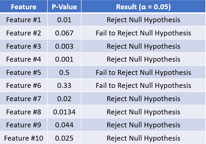
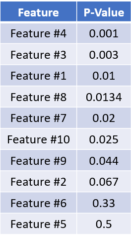
Let’s assume we have 10 features, and we already did our hypothesis testing for each feature. What we get could be shown in the image below.
Normally, when we get the P-value < 0.05, we would Reject the Null Hypothesis and vice versa. Although, just like I outline before that, we might see a significant result due to a chance. That is why we would try to correct the α to decrease the error rate. In this example, we would do it using Bonferroni Correction.
Bonferroni Correction method is simple; we control the α by divide it with the number of the testing/number of the hypothesis for each hypothesis.
If we make it into an equation, the α Bonferroni is the significant α divided by m (number of hypotheses).
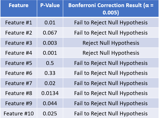
In our image above, we have 10 hypothesis testing. It means we divide our significant level of α 0.05 by 10, and the result is 0.005. If we apply it to our testing above, it will look like this.
With Bonferroni Correction, we get a stricter result where seven significant results are down to only two after we apply the correction.
Holm–Bonferroni correction method
Bonferroni Correction is proven too strict at correcting the α level where Type II error/ False Negative rate is higher than what it should be. That is why there are many other methods developed to alleviate the strict problem. One of the examples is the Holm-Bonferroni method.
In this method, the α level correction is not uniform for each hypothesis testing; instead, it was varied depending on the P-value ranking. By ranking, it means a P-value of the hypothesis testing we had from lowest to highest.
Let’s try to rank our previous hypothesis from the P-value we have before. The rank should look like this.
After we rank the P-value, we would the correct α level and test the individual hypothesis using this equation below.
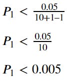
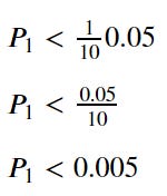
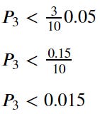
Where k is the ranking and m is the number of hypotheses tested. In the above example, we test ranking 1 for the beginning. If we put it into an equation, it would look like this.
Our first P-value is 0.001, which is lower than 0.005. It means we can safely Reject the Null Hypothesis. Then we move on to the next ranking, rank 2.
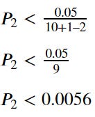
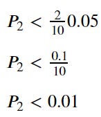
This time, our second P-value is 0.003, which is still lower than 0.0056. This means we still Reject the Null Hypothesis and move on to the next rank.
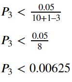
In the third rank, we have our P-value of 0.01, which is higher than the 0.00625. In this case, we Fail to Reject the Null Hypothesis. When this happens, we stop at this point, and every ranking is higher than that would be Failing to Reject the Null Hypothesis. It means from rank 3to 10; all the hypothesis result would be Fail to Reject the Null Hypothesis.
Coincidentally, the result we have are similar to Bonferroni Correction. Sometimes it is happening, but most of the time, it would not be the case, especially with a higher number of hypothesis testing.
Above are examples of what FWER methods are. There are still many more methods within the FWER, but I want to move on to the more recent Multiple Hypothesis Correction approaches.
False Discovery Rate correction
With a skyrocketing number of hypotheses, you would realize that the FWER way of adjusting α, resulting in too few hypotheses are passed the test. That is why a method developed to move on from the conservative FWER to the more less-constrained called False Discovery Rate (FDR).
The way the FDR method correcting the error is different compared to the FWER. While FWER methods control the probability for at least one Type I error, FDR methods control the expected Type I error proportion. In this way, FDR is considered to have greater power with the trade-off of the increased number Type I error rate.
Benjamini–Hochberg (BH) correction method
Benjamini-Hochberg (BH) method or often called the BH Step-up procedure, controls the False Discover rate with a somewhat similar to the Holm–Bonferroni method from FWER. The process is similar because the BH method ranks the P-value from the lowest to the highest. The hypothesis is then compared to the α level by the following equation.
Where k is the rank and m is the number of the hypotheses. If you realize, with this method, the alpha level would steadily increase until the highest P-value would be compared to the significant level. Let’s take our previous data for our example.
If we take the rank 1 P-value to the equation, it will look like this.
Our first P-value is 0.001, which is lower than 0.005. It means we can safely Reject the Null Hypothesis. Then we move on to the next ranking, rank 2.
The second P-value is 0.003, which is still lower than 0.01. This means we still Reject the Null Hypothesis and move on to the next rank.
The rank 3 P-value is 0.01, which is still lower than 0.015, which means we still Reject the Null Hypothesis. We keep repeating the equation until we stumbled into a rank where the P-value is Fail to Reject the Null Hypothesis. On our data, it would be when we in rank 8.
Multiple Hypothesis Correction using MultiPy
I hope you already understand the basic concept of Multiple Hypothesis Correction because, in these parts, I would show you the easier parts; Using Python Package to do our Multiple Hypothesis Correction.
Luckily, there is a package for Multiple Hypothesis Correction called MultiPy that we could use. Let’s get started by installing the necessary package.
pip install multipyWith this package, we would test various methods I have explained above. In this example, I would use the P-values samples from the MultiPy package. Let’s get started.
import pandas as pd#Import the data samplesfrom multipy.data import neuhaus#Import the FWER methods from multipy.fwer import bonferroni, holm_bonferroni#Import the FDR methods (LSU is the other name for BH method)from multipy.fdr import lsuWhen we have all the required package, we will start testing the method. First, I would set up the P-values data sample.
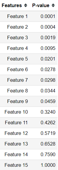
pvals = neuhaus()df = pd.DataFrame({'Features': ['Feature {}'.format(i) for i in range(1,len(pvals)+1 )], 'P-value':pvals})The data samples already provided us the P-value example; what I did is just created a Data Frame object to store it.
Now, let’s try the Bonferroni Correction to our data sample.
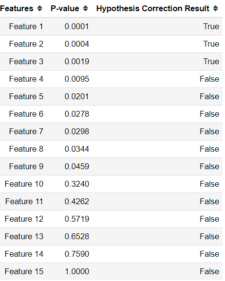
#Set the alpha level for your desired significant leveldf['Hypothesis Correction Result'] = bonferroni(pvals, alpha = 0.05)With the function from MultiPy, we end up either with True or False results. True means we Reject the Null Hypothesis, while False, we Fail to Reject the Null Hypothesis.
From the Bonferroni Correction method, only three features are considered significant. Let’s try the Holm-Bonferroni method to see if there is any difference in the result.
df['Hypothesis Correction Result'] = holm_bonferroni(pvals, alpha = 0.05)No change at all in the result. It seems the conservative method FWER has restricted the significant result we could get. Let’s see if there is any difference if we use the BH method.
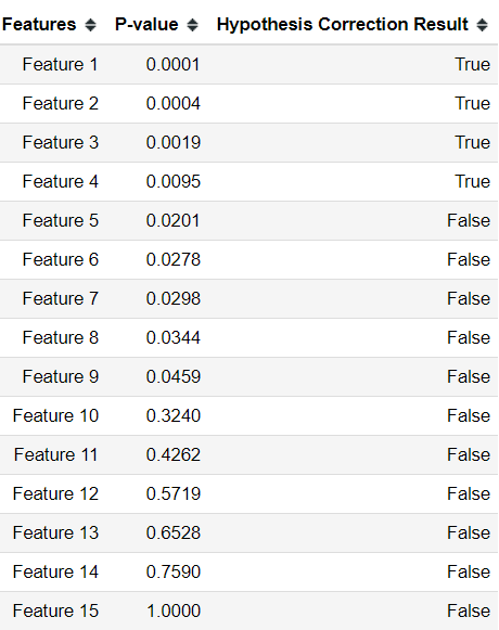
#set the q parameter to the FDR rate you wantdf['Hypothesis Correction Result'] = lsu(pvals, q = 0.05)The less strict method FDR resulted in a different result compared to the FWER method. In this case, we have four significant features. The FDR is proven to laxer to find the features, after all.
If you want to learn more about the methods available for Multiple Hypothesis Correction, you might want to visit the MultiPy homepage.
Conclusion
Hypothesis Testing is a must-know knowledge for a Data Scientist because it is a tool that we would use to prove our assumption.
The problem with Hypothesis Testing is that when we have multiple Hypothesis Testing done simultaneously, the probability that the significant result happens just due to chance is increasing exponentially with the number of hypotheses.
To solve this problem, many methods are developed for the Multiple Hypothesis Correction, but most methods fall into two categories; Family-Wise error rate (FWER) or FDR (False Discovery Rate).
For an easier time, there is a package in python developed specifically for the Multiple Hypothesis Testing Correction called MultiPy.
I hope it helps!


