Python Packages for Studying Causal Learning - NBD Lite #37

Learn cause and effect analysis with these packages

Causal Analysis is a field within experimental statistics that aims to prove and establish the cause-and-effect relationship.

In statistics, using statistical algorithms to infer causality within the dataset under the strict assumption is called Exploratory causal Analysis (ECA).

ECA, in turn, is a way to prove causation with more controllable experimentations and not only based on correlation.

We often need to prove the Counterfactual—a different condition under other circumstances. The problem is that we can only approximate the Causal Effect, not the Counterfactual.

Image by Author.

Causal Analysis is already a different field of learning in data science because it inherently differs from prediction in machine learning modeling.

We could predict the ML result from the existing data but never what came outside of the existing data.

To learn more about Causal Analysis, this article will present you with 4 Python Packages you could use for learning material. Let’s get into it.

---

1. Causalinference

Causalinference is a Python package that provides various statistical methods for causal Analysis. It is a simple package that was used for basic causal analysis learning. The main features of these packages include:

• Propensity score estimation and subclassification

• Improvement of covariate balance through trimming

• Estimation of treatment effects

• Assessment of overlap in covariate distributions

We can find the explanation on their web page for a longer explanation regarding each term.

Let’s try out the Causalinference package. For starters, we need to install the package.

pip install causalinference

After the installation finishes, we will try to implement a causal model for causal Analysis.

We will use the random data from the causal inference package.

from causalinference import CausalModel
from causalinference.utils import random_data#Y is the outcome, D is treatment status, and X is the independent variableY, D, X = random_data()
causal = CausalModel(Y, D, X)

The CausalModel class would analyze the data.

We need to do a few more steps to acquire important information from the model. First, let’s get the statistical summary.

print(causal.summary_stats)

Image by Author

By using the summary_stats attribute, we would acquire all the basic information of the dataset.

The central part of causAnalysissis is acquiring the treatment effect information.

The simplest one is to use the Ordinary Least Square method.

causal.est_via_ols()
print(causal.estimates)

Image by Author

ATE, ATC, and ATT stand for Average Treatment Effect, Average Treatment Effect for Control, and Average Treatment Effect for Treated, respectively.

We could use this information to assess whether the treatment has an effect compared to the control.

Using the propensity score method, we could also get information regarding the probability of treatment conditional on the independent variables.

causal.est_propensity_s()
print(causal.propensity)

Image by Author

Using the propensity score method, we could assess the probability of the treatment given the independent variables.

There are still many methods you could explore and learn from. I suggest you visit the Causalinference web page to learn more.

---

2. Causallib

Causallib is a Python package for Causal Analysis developed by IBM. The package provides a causal analysis API unified with the Scikit-Learn API, which allows a complex learning model with the fit-and-predict method.

The Causallib package has a good number of example notebooks that we could use for our learning process.

Image by Author

Then, let’s try to use the causallib package for our learning. First, we need to install the package.

pip install causallib

After that, we will use an example dataset from the causallib package and estimate the causaAnalysisis using the Scikit-Learn model.

from sklearn.linear_model import LogisticRegression
from causallib.estimation import IPW 
from causallib.datasets import load_nhefsdata = load_nhefs()
ipw = IPW(LogisticRegression())
ipw.fit(data.X, data.a)
potential_outcomes = ipw.estimate_population_outcome(data.X, data.a, data.y)
effect = ipw.estimate_effect(potential_outcomes[1], potential_outcomes[0])

The above code would load a follow-up study regarding the effect of smoking on health. We used the Logistic Regression model as a Causal Model to establish and assess the causal effect.

Let’s check what happens to the treatment’s potential outcome and effect.

print(potential_outcomes)

Image by Author

Checking the potential outcomes, we can see that the average weight difference if everyone had quit smoking (1) is 5.38 kg.

The average weight difference if everyone smokes continuously (0) is 1.71kg.

This means we have average weight differences of around 3.67 kg. So, we could conclude that smoking would decrease weight gain by around 3.67 kg.

For more information and learning material, please visit the notebook on the Causallib page.

---

3. Causalimpact

Causalimpact is a Python package for Causal Analysis that estimates the causal effect of a time series intervention. The analysis shows the difference between the treatment before and after the fact.

Causalimpact would analyze the response time series (e.g., clicks, drug effect, etc.) and a control time series (your response but in a more controlled environment) with the Bayesian structural time-series model.

This model predicts the counterfactual if the intervention never happens), and then we could compare the result.

Let’s start to use the package by installing it.

pip install causalimpact

After installing the package, let’s create simulated data. We would create an example dataset with 100 observations, with an intervention effect after timepoint 71.

import numpy as np
from statsmodels.tsa.arima_process import arma_generate_sample
from causalimpact import CausalImpactnp.random.seed(1)x1 = arma_generate_sample(ar=[0.999], ma=[0.9], nsample=100) + 100
y = 1.2 * x1 + np.random.randn(100)y[71:100] = y[71:100] + 10
data = pd.DataFrame(np.array([y, x1]).T, columns=["y","x1"])
pre_period = [0,69]
post_period = [71,99]

Image by Author

Above, we acquire a dependent variable (y) and an independent variable (x1). Usually, we would have more than one independent variable, but let’s stick with the current data.

Let’s run the analysis analysis data. We need to specify the period before and after the intervention.

impact = CausalImpact(data, pre_period, post_period)
impact.run()
impact.plot()

Image by Author

The plot above gives us three sets of information. The top panel shows the actual data and a counterfactual prediction for the post-treatment period. The middle panel shows the difference between actual data and counterfactual predictions, which is the pointwise causal effect.

The bottom panel is a plot of the cumulative effect of the intervention, where we accumulate the pointwise contributions from the middle panel.

If we want to gain information from each data point, we could use the following code.

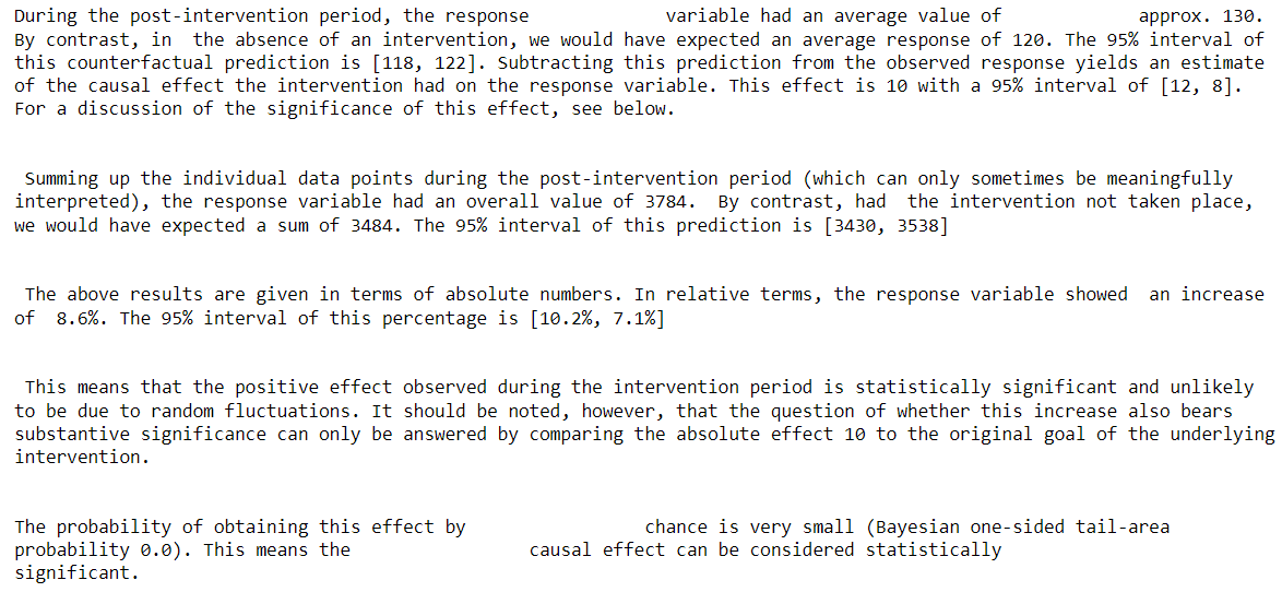
impact.inferences

Image by Author

Also, a summary result is acquired via the following code.

impact.summary()

Image by Author

The summary allowed us to assess whether the intervention had a causal effect.

You could use the following code if you want a more detailed report.

impact.summary(output = 'report')

Image by Author

If you want to learn more about the time-intervention causal analysis, check out their documentation page.

---

4. DoWhy

DoWhy is a Python package that provides state-of-the-art causal analysis with simple API and complete documentation.

If we visit the documentation Page, DoWhy did the causal analysis analysis:

1. Model a causal inference problem using assumptions we create,

2. Identify an expression for the causal effect under the assumption,

3. Estimate the expression using statistical methods,

4. Verify the validity of the estimate.

Let’s try to initiate a causal analysis with the DoWhy package. First, we must install it by running the following code.

pip install dowhy

After that, we would use the randomized dataset from the DoWhy package as a sample dataset.

from dowhy import CausalModel
import dowhy.datasets# Load some sample data
data = dowhy.datasets.linear_dataset(
    beta=10,
    num_common_causes=5,
    num_instruments=2,
    num_samples=10000,
    treatment_is_binary=True)

First, given a graph and assumption we create, we could develop it into the causal model.

Create a causal model from the data and given graph.
model = CausalModel(
    data=data["df"],
    treatment=data["treatment_name"],
    outcome=data["outcome_name"],
    graph=data["gml_graph"])model.view_model()

Image by Author

Next, we need to identify the causal effect with the following code.

#Identify the causal effect
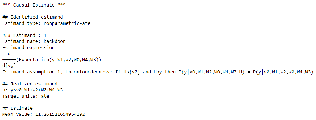
estimands = model.identify_effect()

Image by Author

We identify a causal effect, and then we need to estimate how strong the effect is statistically.

estimate = model.estimate_effect(identified_estimand,                              method_name="backdoor.propensity_score_matching")

Image by Author

Lastly, the causal effect estimation is based on the data’s statistical estimation, but the causality itself is not based on the data; rather, it is based on our previous assumptions. We need to check the assumption validity with the robustness check.

refute_results = model.refute_estimate(identified_estimand, estimate,                                     method_name="random_common_cause")

Image by Author

With that, we completed the causal analysis. The analysis uses this information to decide whether the treatment has a causal effect.

DoWhy documentation offers vast learning material; you should visit the web page to learn more.

---

That’s all my top Python packages for learning Causal Analysis.

Are there any more things you would love to discuss? Let’s talk about it together!

👇👇👇

---